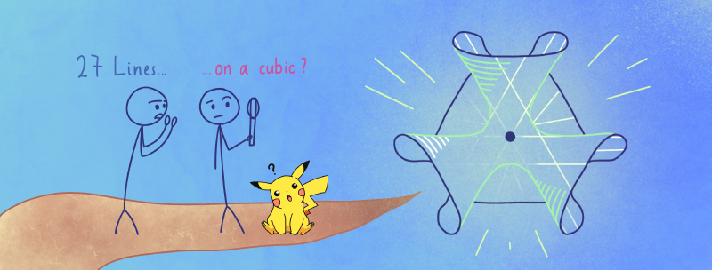
Algebraic geometry has always been one of my dream topics to study since the first time I’m exposed to the notion. Ravi Vakil, being the author of one of the greatest notes in AG, quotes the following in Chapter 27:
Wake an algebraic geometer in the dead of night, whispering: “27”. Chances are, he will respond: “lines on a cubic surface”. – R. Donagi and R. Smith, (on page 27)
Well, it certainly occurs to me that 27 carries a special meaning to algebraic geometrists. Over the summer I’m lucky to have the chance to do a UROP with Prof. Johannes Nicaise, and he suggested that I should embark a journey aiming to understand this statement, which is exactly what I did and what I will try to reconstruct in this post.
Note: This is the first half of a two-part post on this topic. For the other half, see here.
Part 1: The tools
Before delving into the intricacies of the 27 lines, we need to arm ourselves with some tools. We ought to answer questions like: What is a cubic surface? What is smooth? Where exactly do they live? What are lines? What is 27? What even is maths?
Let us start with the easiest question to answer: what is the ambient space of a cubic surface?
The ambient space
In its easiest form, we want to consider the following type of objects:
We call $$\mathbb{A}^n:=\lbrace (a_1,\ldots,a_n):a_i\in K ~\text{for}~i=1,\ldots,n\rbrace$$ the affine $n$-space over $K$. For a subset $S\subseteq K[x_1,x_2,\ldots,x_n]$ of polynomials, we call $$V(S):=\lbrace x\in \mathbb{A}^n: f(x)=0~\text{for all}~f\in S\rbrace\subseteq \mathbb{A}^n$$ the zero locus of $S$. Subsets of $\mathbb{A}^n$ of this form are called affine varieties.
The main idea is that Algebraic Geometry study objects defined via polynomials; for example, a parabola is the zero locus of the polynomial $y-x^2$:

This is natural, but is not good enough: it turns out that these affine varieties are never compact in the classical topology (unless they consist of finitely many points). We don’t want this because some varieties end up having no points, so counting intersections on our cubics and all sorts of related stuff fail.
The way out of this is to consider a “compactification” of $\mathbb{A}^n$. Suppose you have two equations that originally does not intersect in the affine space, say:
$$x+y=1~~~\text{and}~~~x+y=2.$$
By making the equation homogeneous, i.e. such that all terms have the same degree, we resolve this problem: the new equations are then
$$x+y=z~~~\text{and}~~~x+y=2z,$$
so they intersect at $(x,y,z)=(\lambda,-\lambda,0)$, which we can think of as a “point” infinitely far in the direction of $(1,-1,0)$.

Note that we always get “lines through the origin” as solutions of homogeneous equations (in this particular case, the line is spanned by $(1,-1,0)$), since if $f(x_1,\ldots,x_n)$ is homogeneous then
$$f(x_1,\ldots,x_n)=0~\Longrightarrow~f(\lambda x_1,\ldots,\lambda x_n)=0$$
for any $\lambda\in K$. This motivates the definition of the projective space:
Let $n\in\mathbb{N}$. The projective $n$-space over $K$ is defined as $$\mathbb{P}^n:=(K^{n+1}\setminus\lbrace 0 \rbrace)/\sim$$ where $\sim$ is the equivalence relation $$(x_0,\ldots,x_n)\sim(y_0,\ldots,y_n)~:\Leftrightarrow~x_i=\lambda y_i~\text{for some}~\lambda\in K^{\ast}~\text{and all}~i.$$ The equivalence class of $(x_0,\ldots,x_n)$ will be denoted by $[x_0:\cdots:x_n]\in\mathbb{P}^n$. For a subset $S\subseteq K[x_0,\ldots,x_n]$ of homogeneous polynomials, we call $$V(S):=\lbrace x\in \mathbb{P}^n: f(x)=0~\text{for all}~f\in S\rbrace\subseteq \mathbb{P}^n$$ the zero locus of $S$. Subsets of $\mathbb{P}^n$ of this form are called projective varieties.
Note that we really need the homogeneous condition in the definition of projective zero locus for it to make sense: if not, say $f([x:y])=x+y+1$ when $n=1$, then
$$f([-1:0])=0~~~\text{and}~~~f([1:0])=2,$$
yet $[-1:0]=[1:0]$ in $\mathbb{P}^1$. So the zero locus of $f$ is not well-defined here.
Note: from now on, all fields $K$ in discussion will be an algebraically closed field with characteristic zero, so you may assume $K=\mathbb{C}$.
The Zariski Topology
The next step is to endow a topological structure on every variety. As a result,
- we can view varieties as an object in their own right, instead of an object locked in an ambient space $\mathbb{A}^n$ or $\mathbb{P}^n$.
- we can make sense of topological statements like “the complement of an affine variety is huge”.
We first define a topology on the whole ambient space:
The Zariski topology on $\mathbb{A}^n$ (or $\mathbb{P}^n$) is the topology whose closed sets are exactly the affine (projective) varieties, i. e. the subsets of the form $V(S)$ for some set of polynomials $S$.
As in the definition of $V(\cdot)$, we require that $S$ has to consist of homogeneous polynomials in the projective setting $\mathbb{P}^n$.
Before we check that the Zariski topology indeed forms a topology, let us try to figure out the Zariski topology on $\mathbb{A}^1$ as an example:
We observe that:
- Closed sets of $\mathbb{A}^1=\mathbb{C}$ are of the form $V(S)$ where $S$ consists of single-variable polynomials $f(x)$.
- By the fundamental theorem of algebra, $f(x)$ has at most $\deg f$ roots, so the same holds for $V(S)$: by definition $$x\in V(S)~\Longleftrightarrow~x~\text{is a root of all}~f\in S,$$ so $V(S)$ is finite.
- Hence, the closed sets are either $\mathbb{A}^1$ itself ($V(0)$) or a finite set (including $\emptyset$). Thus, the open sets are $\emptyset$ and $\mathbb{A}^1$ minus set of finite points.
In other words, a picture of a “typical” open set in $\mathbb{A}^1$ might be

i.e. it is everything except a few marked points.
Now, as promised, let us check that this indeed form a topology:
The Zariski topology forms a topology.
Proof. We will only show the result for $\mathbb{A}^n$; the case of $\mathbb{P}^n$ is analogous. It suffices to check the following axioms for a topology:
-
$\emptyset$ and $\mathbb{A}^n$ are closed: We have $\emptyset=V(1)$ and $\mathbb{A}^n=V(0)$, so they are closed by definition.
-
The union of any finite number of closed sets are closed: It suffices to check that the union of two closed sets are closed. Indeed, we shall show that $$V(S_1)\cup V(S_2)=V(S_1S_2)$$ where $S_1S_2:=\lbrace fg:f\in S_1, g\in S_2\rbrace$.
Take $x\in V(S_1)\cup V(S_2)$, then $f(x)=0$ for all $f\in S_1$ or $g(x)=0$ for all $g\in S_2$. In both case this means $$(fg)(x)=0~\text{for all}~f\in S_1~\text{and}~g\in S_2,$$ i.e. $x\in V(S_1S_2)$. This shows $V(S_1)\cup V(S_2)\subseteq V(S_1S_2)$. ($\supseteq$) is similar. -
Any intersection (finite or infinite) of closed sets are closed: Again, one can show similarly (also as an easy exercise) that $$\bigcap_{i\in I} V(S_i)=V\left(\bigcup_{i\in I} S_i\right)$$ for an index set $I$ and $S_i\subseteq K[x_1,\ldots,x_n]$. Hence the intersection is closed.
The three axioms combined shows the desired statement. □
The last thing we have to do is to assign a topology on an arbitrary affine (or projective) variety $X$; but the theory of topology automatically does that for us: The Zariski topology on $X$ will be the subspace topology on $X$, i.e. the closed (or equivalently, open) sets are of the form $X\cap Y$ where $Y$ is closed (open) in $\mathbb{A}^n$ (or $\mathbb{P}^n$).
Again consider $X=V(y-x^2)\subseteq\mathbb{A}^2$, and let $U=X\setminus{(1,1)}$. We claim $U$ is open in $X$:

Indeed, $\tilde{U}=\mathbb{A}^2\setminus{(1,1)}$ is open in $\mathbb{A}^2$ (since it is the complement of the closed set $V(x-1,y-1)$), so $U=\tilde{U}\cap X$ is open in $X$. Note that on the other hand the set $U$ is not open in $\mathbb{A}^2$.
Grassmannians
Now it just remains to introduce one final tool! Unfortunately, this one’s a bit more technical, so bear with me. Recall that a point in $\mathbb{P}^n$ can actually be viewed as a line in $K^{n+1}$, such as $[1:1:0]$ corresponding to the line $\operatorname{Span}(1,1,0)$. In other words, we can view $$\mathbb{P}^n=\lbrace 1\text{-dimensional linear subspaces of}~K^{n+1}\rbrace.$$
Since the definition of projective spaces turned out to be a very useful concept, let us now generalize this and consider instead the sets of $k$-dimensional linear subspaces of $K^{n}$:
Let $n$ be a positive integer, and let $k$ be an integer with $0\leq k\leq n$. We denote by $G(k,n)$ the set of all $k$-dimensional linear subspaces of $K^n$, called the Grassmannian of $k$-planes in $K^n$.
So, by above, $\mathbb{P}^n=G(1,n+1)$. Surprisingly, although $G(k,n)$ seems to be a generalisation of projective spaces, there is actually a natural embedding of $G(k,n)$ into a projective space $\mathbb{P}^N$ for some $N$. Moreover, “points” in $G(k,n)$, i.e. the $k$-dimensional subspaces, can be described using polynomials, so $G(k,n)$ will form a projective variety.
Let us first look at the case of $G(2,n)$. For this to work we will need the algebraic concept of wedge products:
Let $V$ be a $K$-vector space. The $2$-wedge product $\Lambda^2(V)$ is defined as the span of elements of the form ${v}\wedge {w}$ (where ${v},{w}\in V$), subject to the same relations as the tensor product $\otimes$:
- distributive in $V$: $({v}_1+{v}_2)\wedge {w}={v}_1\wedge{w}+{v}_2\wedge{w}$;
- distributive in $W$: ${v}\wedge({w}_1+{w}_2)={v}\wedge{w}_1+{v}\wedge{w}_2$;
- $(\lambda{v})\wedge {w}={v}\wedge (\lambda{w})$.
but with two additional relations:
- ${v}\wedge{v}=0$;
- ${v}\wedge{w}=-{w}\wedge{v}$.
Scalar multiplication is defined by $\lambda\cdot({v}\wedge{w})=(\lambda{v})\wedge {w}={v}\wedge (\lambda{w})$.
If you like, you can phrase this whole definition as saying that $\wedge$ is an alternating bilinear operation. Note that if $V$ has basis $\lbrace e_1,\ldots,e_n\rbrace$, then $\Lambda^2(V)$ has basis $$\lbrace e_i\wedge e_j:i<j\rbrace,$$ so $\dim \Lambda^2(V)={n\choose 2}$.
Similarly, we can define the $k$-wedge product $\Lambda^k(V)$ for any integer $0\leq k\leq n$, where the there are $k-1$ wedges, and swapping any two consecutive components negate the whole wedge. Naturally we have $\dim \Lambda^k(V)={n\choose k}$, where the basis is given by $$\lbrace e_{i_1}\wedge e_{i_2}\wedge \cdots\wedge e_{i_k}:i_1<i_2<\cdots<i_k\rbrace.$$
But why do we need these new bizzare spaces for our discussion? Before we answer that, let’s first look at an explicit computation:
Let $V=K^2$, and let $v=ae_1+be_2,w=ce_1+de_2$. Now let’s compute $v\wedge w$ in $\Lambda^2(V)$:
$$\begin{aligned} {v}\wedge{w} &= (a{e}_1+b{e}_2)\wedge(c{e}_1+d{e}_2) \\ &= ac({e}_1\wedge{e}_1)+bd({e}_2\wedge{e}_2)+ad({e}_1\wedge{e}_2)+bc({e}_2\wedge{e}_1) \\ &=ad({e}_1\wedge{e}_2)+bc({e}_2\wedge{e}_1) \\ &=(ad-bc)({e}_1\wedge{e}_2). \end{aligned} $$
What is $ad-bc$? You might recognize it as the determinant of $\begin{pmatrix}a & b\\ c & d\end{pmatrix}$. Indeed, the wedge product $v\wedge w$ is highly related to the minors of the matrix with rows as $v$ and $w$. This is in fact a general phenomenon:
Let $v_1,\ldots,v_k\in K^n$. Then the $(e_{i_1}\wedge \cdots\wedge e_{i_k})$-coordinates of $v_1\wedge \cdots\wedge v_k$ is the minor of the matrix whose rows are $v_1,\ldots,v_k$ obtained by taking only the $i_1,\ldots,i_k$-th columns.
This fact just follows from the definition of the determinant. To understand the statement, consider the case $k=2$ and $n=3$. Then by writing $v=a_1e_1+a_2e_2+a_3e_3$ and $w=b_1e_1+b_2e_2+b_3e_3$, the matrix is $$\begin{pmatrix}a_1 & a_2 & a_3 \\ b_1 & b_2 & b_3\end{pmatrix}$$ so the fact is saying that the coefficient of, say $e_2\wedge e_3$, is the determinant of the submatrix by deleting the first column, i.e. $a_2b_3-b_2a_3$.
Let’s come back to algebraic geometry now. We define:
Let $0\leq k\leq n$. Since $\dim\Lambda^k K^n={n\choose k}$, we have $\Lambda^k K^n\cong K^{n\choose k}$, and so can be viewed as the projective space $\mathbb{P}^{{n\choose k}-1}$. The Plücker embedding is defined as the map $$\begin{aligned} f:&&G(k,n)&\to \mathbb{P}^{{n\choose k}-1} \\ &&\operatorname{Span}(v_1,\ldots,v_k)&\mapsto v_1\wedge\cdots\wedge v_k\in \Lambda^kK^n. \end{aligned}$$
We have to check that this map $f$ is well-defined, i.e. we have to check:
- $v_1\wedge\cdots\wedge v_k$ will not be zero, or else it is not a point in $\mathbb{P}^{{n\choose k}-1}$.
- Choosing a different basis of the subspace $\operatorname{Span}(v_1,\ldots,v_k)$ does not change the resulting point in $\mathbb{P}^{{n\choose k}-1}$.
These two statements can be resolved by the following lemma:
Let $V=\operatorname{Span}(v_1,\ldots, v_k)$ and $W=\operatorname{Span}(w_1,\ldots, w_k)$. Then:
- $f(V)=0$ if and only if $v_1,\ldots,v_k$ are linearly dependent.
- $f(V)$ and $f(W)$ are linearly dependent in $\Lambda^k K^n$ if and only if $V=W$.
Proof. We will only prove the first statement, and the second one is left as an exercise (in linear algebra). By Fact 7, we have $v_1\wedge \cdots\wedge v_k=0$ iff all maximal minors of the matrix with rows $v_1,\ldots,v_k$ are zero. But this is the case iff this matrix does not have full rank, i.e. iff $v_1,\ldots,v_k$ are linearly dependent. □
So we finally can explain why the wedge product is useful. At first we want to assign a subspace in $G(k,n)$ to a unique point in $\mathbb{P}^N$, but the wedge product does exactly that, since:
- The bilinear conditions guarantee that the same subspace with a different basis still generates the same $v_1\wedge\cdots\wedge v_k$, up to multiplication of a scalar (by Lemma 9(ii)). But then they correspond to the same point in $\mathbb{P}^N$ since scalars are neglected.
- The additional condition $\cdots\wedge v\wedge v\wedge\cdots=0$ guarantee that points in $\mathbb{P}^N$ only correspond to $k$-dimensional subspaces, not the ones with smaller dimensions.
Finally, one can check that this map $f$ is injective (again by Lemma 9(ii)), hence the name “embedding”.
Let us compute some examples of the Plücker embedding to see what it actually is doing:
- The Plücker embedding of $G(1,n)$ simply maps a linear subspace $\operatorname{Span}(a_1e_1+\cdots+a_ne_n)$ to $(a_1:\cdots:a_n)\in \mathbb{P}^{{n\choose 1}-1}=\mathbb{P}^{n-1}$. Hence $G(1,n)=\mathbb{P}^{n-1}$ as expected.
- Consider the subspace $L=\operatorname{Span}(e_1+e_2,e_1+e_3)\in G(2,3)$ of $K^3$. The coordinates of $f(L)$ would be the maximal minors of $$\begin{pmatrix}1 & 1 & 0 \\ 1 & 0 & 1\end{pmatrix},$$ so under the basis $\lbrace e_1\wedge e_2,e_1\wedge e_3,e_2\wedge e_3\rbrace$ the corresponding point in $\mathbb{P}^{{3\choose 2}-1}=\mathbb{P}^2$ is $[-1:1:1]$.
Pictorially, we can now see $G(k,n)$ as an object living in $\mathbb{P}^{N-1}$, whose points parameterise $k$-dimensional subspaces in $K^n$:

But we are still yet to see that it is a closed subset, i.e. a projective variety. As an idea, the proof is purely algebraic, by noticing that the image of the Plücker embedding are the set of pure tensors, i.e. the wedge products that doesn’t involve sums. This then turns out to be a polynomial condition, so $G(k,n)$ is closed. We will omit the proof, since it doesn’t contribute much to our discussion. Readers who want to know the whole process might consult here.